Let

be the cardinal cubic spline
space with distance

between consecutive knots, on the interval
![$ [0,1]$](img311.png)
. This is
a subspace of dimension

, which we span using a
B-spline basis
The functions

in

are obtained by
translations of a prototype function
and the restriction to the interval
. A
few of such functions
are plotted in the left graph of Fig.
3.
Figure 3:
Left graph: cubic B spline functions, in the rage
![$ x
\in [0.1, 0.3]$](img1.png) ,
from the set spanning the space of the signal response.
Right graph: tree of the functions spanning the space of the
background.
,
from the set spanning the space of the signal response.
Right graph: tree of the functions spanning the space of the
background.
|
|
Taking, randomly, 30 B-splines
 from
from
 we simulate a signal by a weighted superposition of such functions,
i.e.,
we simulate a signal by a weighted superposition of such functions,
i.e.,
![$\displaystyle f_{\cal{V}}(x)=\sum_{i=1}^{30} c_{\ell_i} B_{\ell_i}(x),\quad x\in [0,1],$](img320.png) |
(15) |
with the coefficients

randomly chosen from
.
We simulate a background by considering it belongs
to the subspace
 spanned by the set of functions
A few functions from this set are plotted in the right
graph of Fig.
3 (normalized to unity on
![$ [0, 1])$](img323.png)
.
The background,

is generated by
the linear combination
 |
(16) |
To simulate the data
we have perturbed the superposition of

and

, by
`very small' Gaussian errors (of variance up to

the value
of each data point). The simulated data are plotted
in the left graph of Fig.
4.
This example is very illustrative of how sensitive to
errors the oblique projection is.
The subspace we are dealing with are disjoint: the
last five singular values of operator
 (c.f. (11))
are:
(c.f. (11))
are:
while the first is
.
The smallest singular value cannot be considered a
numerical representation of zero, when the calculations are being
carried out in double precision arithmetic. Hence, one can assert that
the condition
is fulfilled.
However, due to the three small singular values
the oblique projector along
onto the whole subspace
is very unstable, which causes the failure to correctly separate signals
in
from the background. The result of applying
the oblique projector onto the signal of the left graph is
represented by the broken line in the right graph.
As can be observed, the projection
does not yield the required signal, which is
represented by the continuous dark line in the same graph.
Now, since the spectrum of singular values has a clear jump
(the last three singular values are far from the previous ones)
it might seem that one could regularize the projection by truncation
of singular values. Nevertheless, such a methodology turns out to be not
appropriate for the present problem, as it does not yield the correct
separation.
Propositions
3 below analyzes the effect that regularization
by truncation of singular values produces in the resulting
projection.
Figure 4:
Left graph: signal plus background.
Right graph: the dark continuous line corresponds to the signal to be
discriminated from the one in the left graph. The broken line corresponds
to the approximation resulting from the oblique projection.
The three closed lines correspond to the approximations obtained by
truncation of one, two, and three singular values.
|
|
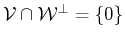
Proposition 3
Truncation of the expansion (13) to consider up to  terms,
produces an oblique projector along
terms,
produces an oblique projector along
 , with
 and
and
 onto
onto
 .
.
The proof of these propositions can be found in [
7]
Appendix B. For complete studies of a projector
when
see [
8] and [
9].
This example illustrates, very clearly, the need for nonlinear
approaches: We know that a unique and stable solution does exist, since
the signal which is to be discriminated from the background
actually belongs to a subspace of the given spline space, and
the construction of the oblique projectors onto such a subspace
is well posed. Whoever, the lack of knowledge
about the subspace prevents the separation of the signal components
by a linear operation. A possibility to tackle the
problem is to transform it into the one of finding
the subspace to which the sought signal component belongs to.
In this way the problem can be addressed by nonlinear techniques.

![\includegraphics[width=8cm]{spli2.eps}](img316.png)
![\includegraphics[width=8cm]{gbac.eps}](img317.png)
![\includegraphics[width=8cm]{exasigo3.eps}](img333.png)
![\includegraphics[width=8cm]{exatrun2.eps}](img334.png)