Highly Nonlinear Approximations for Sparse Signal Representation

Next: Application to sparse signal Up: Adaptive non-uniform B-spline dictionaries Previous: Background and notations
Building B-spline dictionaries
Let us start by recalling that an extended partition with single inner knots associated with
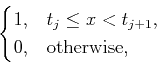 |
|||
 |
The following theorem paves the way for the construction of dictionaries for
Theorem 2
Let
 be partitions of
 ![$ [c,d]$](img495.png) and
and
 . We denote the B-spline basis for
 as
as
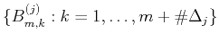 .
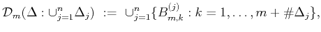
Accordingly, a dictionary,
.
Accordingly, a dictionary,
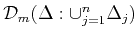 , for
, for
 can be
constructed as
can be
constructed as
 so as to satisfy
 When
When  ,
,
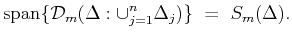
 is reduced to the
B-spline basis of
.
is reduced to the
B-spline basis of
.
Remark 4
Note that the number of functions in the above defined dictionary is
equal to
 , which is larger than
 . Hence, excluding the trivial case
, the dictionary constitutes a redundant dictionary for
.
. Hence, excluding the trivial case
, the dictionary constitutes a redundant dictionary for
.
According to Theorem 2, to build a dictionary for
![\includegraphics[width=8cm]{2-1.eps}](img540.png)
![\includegraphics[width=8cm]{re1-3.eps}](img541.png)
![\includegraphics[width=8cm]{1.eps}](img542.png)
![\includegraphics[width=8cm]{re2-3.eps}](img543.png)
|

This project is supported by EPSRC (EP/D062632/1)
