Oblique projectors in the context of
signal reconstruction were introduced in
[2] and further analyzed in [3].
The application to signal splitting,
also termed structured noise filtering,
amongst a number of other applications,
is discussed in [4]. For advanced
theoretical studies of oblique projector operators
in infinite dimensional spaces see [5,6].
We restrict our consideration to numerical constructions
in finite dimension, with the aim of addressing
the problem of signal splitting when the problem is ill posed.
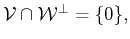
Given  and
and
 disjoint, i.e., such that
 in order to provide a prescription for
constructing
in order to provide a prescription for
constructing
 we proceed as follows. Firstly we
define
we proceed as follows. Firstly we
define  as the direct sum of and
, which we express as
as the direct sum of and
, which we express as
Let
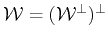
be the orthogonal complement
of
in
. Thus we have
The operations

and

are termed direct and
orthogonal sum, respectively.
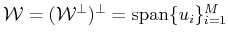
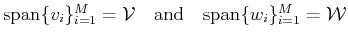
Considering that
 is a spanning set for
a spanning set for
is a spanning set for
a spanning set for  is obtained as
Denoting as
 the standard orthonormal basis in
 ,
i.e., the Euclidean inner
product
,
i.e., the Euclidean inner
product
 , we
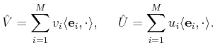
define the operators
, we
define the operators
 and
and
 as
as
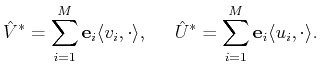
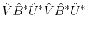
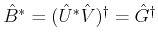
Thus the adjoint operators

and

are
It follows that

and
hence,
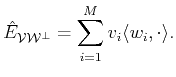
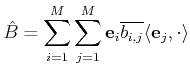
defined as:
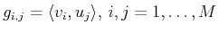
is self-adjoint and its matrix representation,

, has elements
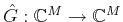
From now on we restrict our signal space to be
,
since we would like to build the oblique projector
onto
and
along
having the form
 |
(3) |
Clearly for the operator to map to zero every vector in
the dual vectors

must span
. This entails that for
each

there exists a set of coefficients

such that
 |
(4) |
which guarantees that every
is orthogonal to all vectors in
and therefore
is included in the null space of
.
Moreover, since every signal,

say, in
can be written as
with

and

,
the fact that

implies

. Hence,

,
which implies that the null space of
restricted to
is
.
In order for
to be a projector it is necessary that
 .
As will be shown in the next
proposition, if the coefficients
.
As will be shown in the next
proposition, if the coefficients  are the matrix
elements of a generalised inverse of the matrix
this condition is fulfilled.
are the matrix
elements of a generalised inverse of the matrix
this condition is fulfilled.
Proposition 1
If the coefficients in (4) are the matrix elements of a
generalised inverse of the matrix , which has elements
 , the operator
in (3) is a projector.
, the operator
in (3) is a projector.
Proof.
For the measurement vectors in (
4) to yield a projector of the
form (
3), the corresponding operator should be idempotent, i.e.,
 |
(5) |
Defining
 |
(6) |
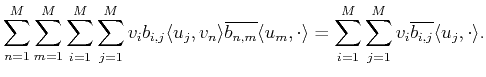
and using the operators

and
, as given above, the
left hand side in (
5) can be expressed as
 |
(7) |
and the right hand side as
 |
(8) |
Assuming that

is a generalised inverse of

indicated as
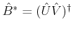
it satisfies
(c.f. Section
![[*]](crossref.png)
)
 |
(9) |
and therefore, from (
7), the right hand side of (
5)
follows. Since
and

, we have

.
Hence, if the elements
determining

in
(
6) are the matrix elements of a generalised inverse
of the matrix representation of

, the corresponding vectors

obtained by (
4) yield an operator of
the form (
3), which is an oblique projector.

Proof.
given in (
3) can be recast, in terms of operator
and
, as:
Applying

both sides of the equation we obtain:
which is a well known form for the orthogonal projector
onto

.
Remark 2
Notice that the operative steps for constructing
an oblique projector are equivalent to those for
constructing an orthogonal one. The difference being that in
general the spaces
 are different.
For the special case
are different.
For the special case  ,
,
 , both sets of
vectors span and
we have an orthogonal projector onto along
, both sets of
vectors span and
we have an orthogonal projector onto along
 .
.
Subsections